Acerca de

COD Reduction

In Wastewater

AI Project

Motivation

I am always curious whether anyone has ever thought about how clean is our every day consumed water?

Or, more importantly, how clean is our drinking water, which would directly affect our health? And, how clean is "clean"?

In the year 2020 at Nan Ya Plastics Corp., I ran into such an opportunity to study how to manage pollutants in wastewater, and here is what I found out.

Problems

During the production of all sorts of plastic, a large amount of sewage is inevitably produced.

If we don't clean up this wastewater, it will profoundly pollute our mother earth, destroy the natural environment and damage our health.

How to measure the pollutants

First of all, we need to define what it means by wastewater or rather polluted water.

An industry-standard index, COD, is used to measure the pollutant. The higher the COD index, the more severe the water is polluted, and it costs more to clean it up.

# Ｗhat is COD?

COD, Chemical Oxygen Demand, is commonly used to represent the degree of pollution in industrial wastewater. It is the amount of oxygen needed to oxidize the organic matter present in water.

High levels of wastewater COD indicate concentrations of organics that can deplete dissolved oxygen in the water, leading to negative environmental and regulatory consequences. To help determine the impact and ultimately limit the amount of organic pollution in water, COD is an essential measurement.

Take Actions

To deal with the wastewater issue, we need to build a testing model to determine how to best reduce the pollutants and COD. After understanding the background of the process, instead of building up an actual entity modeling method like the company always did, which is extremely high cost, time-consuming, and most importantly, non-scalable, I recommend using AI modeling.

AI modeling could tremendously reduce the cost, be highly flexible to control variables hence scalable, and produce more accurate and swift results.

In this way, we successfully reduced COD concentration from 45000 ppm to 30000 ppm in wastewater.

Below is my model building process and project code. Let's take a look!

Manufacturing Process Introduction

The chemical reaction of PTA + EG

I conducted data analysis in cooperation with site engineers. With their help and the domain know-how, I was able to collect the factory data of polyester film and understand the manufacturing production process.

The raw materials of film products are Pure Terephthalic Acid (PTA) and Ethylene Glycol (EG), which undergo esterification reaction during the production process. In addition to BHET and water, the products after the reaction also contain odorous organic compounds, such as Low-molecular-weight aldehydes, which would cause high COD concentration.

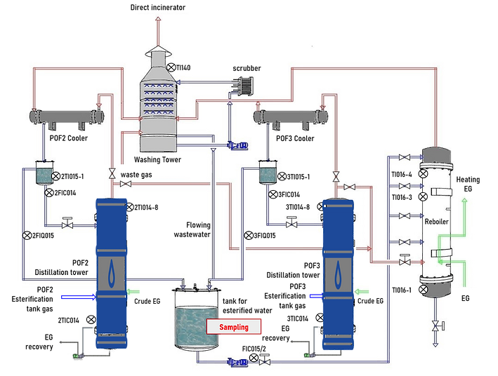
Where would COD be measured ?

The red mark labeled as "Sampling"is where the COD concentration is measured.

The inputs (X variables, independent variable) that are related to the COD sampling point (y variable, target variable) are:

['batch', 'yield', '3DRC004.PV', '3FIC007.PV', '3TIC020', '3FIC020.PV', '3FIC023.PV', '3PIC020.PV', '3PIC023.PV', '3FIC045', '3FIC014', '3TI015-1', '3TI014-8', '3FIQ015.PV']

The flow of wastewater would flow through all these point and then measured at "Sampling" point. Some points are not shown on the figure above.

And what does the meaning of these inputs ?

The English letter after the first number represents the nature of this input.

"F" means flow volume

"T" means temperature

"P" means pressure

About the collective data

After deleting the data with the unstable manufacturing process condition, a total of 200 pieces of data are collected from Jan 2019 to Sep 2020.

COD concentration requires manual evaluation, which is really time-consuming, so the data is only collected once a day; therefore, the speed of collecting data was very slow.

Although the amount of data was not that much, We still found the pattern behind the scenes and gave valuable suggestion.

Modeling process

I think that building a model is a process of constant adjustment, there is no a fixed rule to obey, so it is worth keeping trying different combination of data processing techniques to improve the results.

Data
Cleaning

Exploratory
Data Analysis

Data
Transformation

Feature
Engineering

Predictive
Modeling

Import packages

In [1]:

# data analysis

import numpy as np
import pandas as pd

# visualization

import seaborn as sns

import matplotlib.pyplot as plt

from scipy.stats import skew
from statsmodels.graphics.gofplots import qqplot

%matplotlib inline

# display format

import warningswarnings.filterwarnings('ignore')

np.set_printoptions(suppress =True, precision=4)
pd.options.display.float_format = '{:.4f}'.format

In [2]:

# standardization

from sklearn.preprocessing import MinMaxScaler

from sklearn.preprocessing import StandardScaler

from sklearn.preprocessing import RobustScaler

from sklearn import preprocessing

# evaluation metrics

import math
from sklearn import metrics
from sklearn.metrics import mean_squared_error
from sklearn.metrics import mean_absolute_error, r2_score

from sklearn.metrics import confusion_matrix

import statsmodels.api as sm

# machine learning

from sklearn.model_selection import train_test_split

from xgboost import XGBRegressor
from xgboost.sklearn import XGBClassifier
from sklearn.svm import SVR
from sklearn.linear_model import LinearRegression, Ridge, Lasso, ElasticNet, HuberRegressor
from sklearn.ensemble import RandomForestRegressor, RandomForestClassifier

Input Data

The original data format is not the standard structure, so I format it with python programming.

There is one advantage to process data programmatically rather than manually in excel : when site engineers update the data and give you a brand-new excel, you don't have to manually adjust the format again.

In [3]:

ori_data = pd.read_excel (r'C:\Users\n000173664\Documents\Python Scripts\DataAnalysis\COD_3\CODdata_20200905.xlsx',sheet_name='POF3')
ori_data.head()

In [4]:

# Organize data into structured form
ori_data.columns = ori_data.iloc[0]
ori_data.columns = ori_data.columns.fillna('Datetime')
ori_data = ori_data.drop([0], axis=0)
ori_data = ori_data.drop(['EG處理前'], axis=1)

# Translate to English
ori_data.rename(columns = {"COD處理前" : "COD_before"}, inplace = True) # target variable (y)
ori_data.rename(columns = {"批號" : "batch"}, inplace = True)
ori_data.rename(columns = {"產量" : "yield"}, inplace = True)

# set datetime
ori_data.Datetime = pd.to_datetime(ori_data.Datetime, errors ='coerce') # errors='coerce' fill in NaN
ori_data.set_index('Datetime', inplace = True)

# Turn to numeric except batch
for col in ori_data.columns.drop(['batch']):
ori_data[col] = pd.to_numeric(ori_data[col], errors ='coerce')
ori_data.head()

Check the columns:

In [5]:

ori_data.columns

Index(['COD_before', 'batch', 'yield', '3DRC004.PV', '3FIC007.PV', '3TIC020', '3FIC020.PV',

'3FIC023.PV', '3PIC020.PV', '3PIC023.PV', '3FIC045', '3FIC014', '3TI015-1', '3TI014-8',

'3FIQ015.PV'], dtype='object', name=0)

Make a copy:

In [6]:

df = ori_data.copy()

Define Evaluation Metrics

Let us now define the evaluation error metrics for evaluating the performance of our regression predictive models.

What kind of error metrics we used?

Mean Absolute Percentage Error (MAPE)
MAPE is the mean or average of the absolute percentage errors of forecasts.This measure is easy to understand because it provides the error in terms of percentages. Also, because absolute percentage errors are used, the problem of positive and negative errors canceling each other out is avoided.
Root Mean Squared Error (RMSE)
Square root of mean squared error (MSE) has an advantage that the output value you get is in the same unit as the required output variable which makes interpretation of loss easy. But It is not that robust to outliers as compared to MAPE.
R Squared
R Squared indicates how much variation of a dependent variable is explained by the independent variable(s) in a regression model. It indicates how well a regression model predicts responses for new observations. This statistic helps determine when the model fits the original data but is less capable of providing valid predictions for new observations.

We learned that when the RMSE/ MAPE decreases, the model’s performance will improve. But these values alone are not intuitive. When we talk about the RMSE/ MAPE metrics, we do not have a benchmark to compare.

This is where we can use R-Squared metric. R Squared means how good our regression model as compared to a very simple model that just predicts the mean value of target from the train set as predictions.

In [7]:

# define error metrics for regression models

def CalculateError (y_test, y_pred):
rmse = np.sqrt(mean_squared_error(y_test, y_pred))
mape = np.mean(np.abs((y_test.values.reshape(-1) - y_pred.reshape(-1)) / y_test.values.reshape(-1))) * 100
r2 = metrics.r2_score(y_test, y_pred)
return rmse, mape, r2

◼ Build a base model

As with the modeling process mentioned above, I am used to first establish a base model as a benchmark and then try multiple data processing techniques to improve the error metrics. Below are the machine learning models I used in the project.

Linear Regression
Ridge
Lasso
SVR
Random Forest
XGBoost
Huber Regression

In [8]:

# define error metrics for regression models

LR_model = LinearRegression()
Lasso_model = Lasso(alpha=0.001, random_state=1234)
Ridge_model = Ridge(alpha=0.3, max_iter=500)
SVR_model = SVR(kernel='linear')
RF_model = RandomForestRegressor(random_state=50)
XGB_model = XGBRegressor(random_state=5566)
Huber_model = HuberRegressor()

models = [LR_model, Lasso_model, Ridge_model, SVR_model, RF_model, XGB_model, Huber_model]
model_names = ["LR", "Lasso", "Ridge", "SVR", "RF","XGB", "Huber"]

Split Training and Testing data

In [9]:

# exclude target variable and batch

exclude = ['COD_before', 'batch']

X = df.loc[:,df.columns.difference(exclude)]
y = df.loc[:,'COD_before']

X_train, X_test, y_train, y_test = train_test_split(X, y, train_size=0.9, random_state=42)
print(len(X_train))
print(len(y_test))

173

In [10]:

train_result = pd.DataFrame()

for i,model in enumerate(models):
print('(%d)'%(i+1), model.fit(X_train,y_train))

# train

y_train_pred = model.predict(X_train)
train_rmse, train_mape, train_r2 = CalculateError(y_train, y_train_pred)
print('[1] train result \n', 'rmse:', round(train_rmse, 4),'mape:', round(train_mape, 4),'r2:',round(train_r2, 4))
plt.plot(y_train.values, label='y')
plt.plot(y_train_pred, label='y_pred')
plt.legend()
plt.show()

# test
y_test_pred = model.predict(X_test)
test_rmse, test_mape, test_r2 = CalculateError(y_test, y_test_pred)
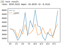
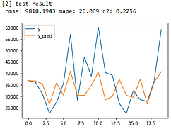
print('[2] test result \n', 'rmse:', round(test_rmse, 4),'mape:', round(test_mape, 4),'r2:',round(test_r2, 4))
plt.plot(y_test.values, label='y')
plt.plot(y_test_pred, label='y_pred')
plt.legend()
plt.show()

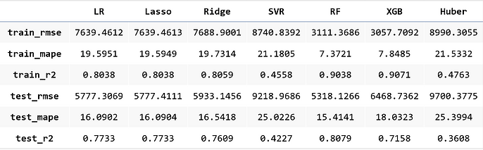
train_result[model_names[i]] = [train_rmse, train_mape, train_r2, test_rmse, test_mape, test_r2]
train_result.index = ['train_rmse', 'train_mape', 'train_r2', 'test_rmse', 'test_mape', 'test_r2' ]

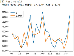
Linear Regression

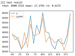
Lasso

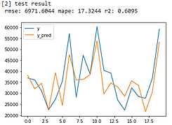
Ridge

SVR

Random Forest

XGBoost

Huber Regression

The model results look just okay. Let’s see how I improve it.

Data Exploration

use data visualization and statistical techniques to describe characteristics of the dataset in order to better understand the nature of the data. These characteristics can include size or amount of data, completeness of the data, correctness of the data, possible relationships amongst data elements or files/tables in the data.

In [11]:

# check data statistics

df.describe()

In [12]:

# check data types and whether the dataset contains missing value

df.info()

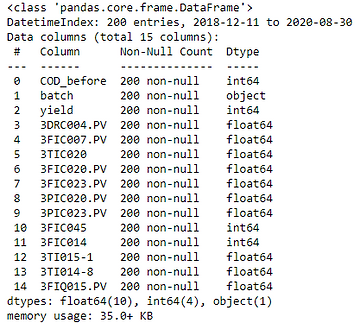
Luckily, there is no missing value, so no need to fill the nan.

Now we can observe the data through data visualization.

In [13]:

# scatter plot

for name in df.columns:
try:
plt.figure(figsize=(20,5))
plt.plot(ori_data[name],'o')
plt.xticks(rotation=45)
plt.title(name)
except:
print(name)

In [14]:

# histogram
others = []
for name in df.columns.drop(['batch']):
try:
sns.distplot(df[name])
plt.figure(figsize=(6,4))
except:
print(name)
others.append(name)
ax = sns.distplot(df[name], rug=True, hist=True, kde_kws={'bw':0.025})

In [15]:

# boxplot

df.plot(kind='box', subplots=True, layout=(3,6), sharex=False, sharey=False, figsize=(20,10),
title='Box Plot for each input variable')
plt.show()

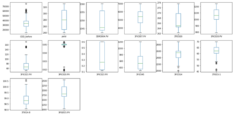
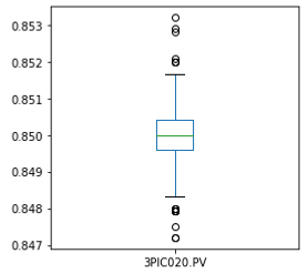
There are some outliers that that can be seen in the graph of 3PIC020.PV.

Simply remove the data with the value below 0.83. After that, we can see the point of 3PIC020.PV follow an approximately normal distribution and the model results improve significantly.

In [16]:

# remove outlier

df = df[df['3PIC020.PV']>0.83]

# histogram

plt.figure(figsize=(4,4))

sns.distplot(df['3PIC020.PV'])

# boxplot

df['3PIC020.PV'].plot(kind='box', subplots=True, sharex=False, sharey=False, figsize=(4,4))
plt.show()

I also tried to remove outliers with the 1.5 x IQR rule or the 5th and 95th percentile values, but it would reduce the data amount significantly, so these methods were not adopted in the end.

Data transformation
& feature engineering

In practice, we often encounter different types of variables in the same dataset. A significant issue is that the range of the variables may differ a lot. Using the original scale may put more weights on the variables with a large range. In order to deal with this problem, we need to apply the technique of features rescaling to independent variables or features of data in the step of data pre-processing.

The goal of applying Feature Scaling is to make sure features are on almost the same scale so that each feature is equally important and make it easier to process by most ML algorithms.

In this dataset, we can easily notice that the variables are not on the same scale.

I tried three types of standardization in this practice.

The most important thing is to use the training parameters and re-use them to scale the test dataset.

When we standardize our training dataset, we need to keep the parameters (mean and standard deviation for each feature). Then, we have to use these parameters to transform our test data and any future data later on.

The reason is that we want to pretend that the test data is “new, unseen data.” We use the test dataset to get a good estimate of how our model performs on any new data. This way could prevent possible data leakage.

Standardization

The result of standardization (or Z-score normalization) is that the features will be rescaled to ensure the mean and the standard deviation to be 0 and 1, respectively.

This technique is to re-scale features value with the distribution value between 0 and 1, and is useful for the optimization algorithms, such as gradient descent, that are used within machine learning algorithms that weight inputs (e.g., regression and neural networks).

In [17]:

# Standardization Initialization

stand_scaler = StandardScaler()

# X_train Normalization
X_train_scale = pd.DataFrame(
data = stand_scaler.fit_transform(X_train),
columns=X_train.columns,
index = X_train.index)

# X_test Normalization
X_test_scale = pd.DataFrame(
data = stand_scaler.transform(X_test),
columns=X_test.columns,
index = X_test.index)

Max-Min Normalization

Another common approach is the so-called Max-Min Normalization (Min-Max scaling). This technique is to re-scales features with a distribution value between 0 and 1. For every feature, the minimum value of that feature gets transformed into 0, and the maximum value gets transformed into 1.

Normalization is good to use when you know that the distribution of your data does not follow a Gaussian distribution. This can be useful in algorithms that do not assume any distribution of the data like K-Nearest Neighbors and Neural Networks.

In contrast to standardization, we will obtain smaller standard deviations through the process of Max-Min Normalization. It implies the data are more concentrated around the mean if we scale data using Max-Min Normalization. As a result, if there are outliers in features, normalizing your data will scale most of the data to a small interval, which means all features will have the same scale. It does not handle outliers well. Standardization is more robust to outliers, and in many cases, it is preferable over Max-Min Normalization.

In [18]:

# Max-Min Normalization Initialization

min_max_scaler = MinMaxScaler(feature_range=(0,1), copy=True)

# X_train Normalization
X_train_scale = pd.DataFrame(
data = min_max_scaler.fit_transform(X_train),
columns=X_train.columns,
index = X_train.index)

# X_test Normalization
X_test_scale = pd.DataFrame(
data = min_max_scaler.transform(X_test),
columns=X_test.columns,
index = X_test.index)

Robust Scaler

Robust Scaler is similar to normalization but it uses the interquartile range instead, so it is robust to outliers.

In [19]:

# Max-Min Normalization Initialization

robust_scaler = RobustScaler()

# X_train Normalization
X_train_scale = pd.DataFrame(
data = robust_scaler.fit_transform(X_train),
columns=X_train.columns,
index = X_train.index)

# X_test Normalization
X_test_scale = pd.DataFrame(
data = robust_scaler.transform(X_test),
columns=X_test.columns,
index = X_test.index)

I tried fitting my models to raw, normalized and standardized data and compare the performance for best results.

In this practice, I found standardization had the best performance.

The following figure demonstrates a simple example showing the data distribution results of the three feature scaling methods after performing the data transformation.

There is a simple but important concept, which many people misunderstand (I was also confused as a beginner). Contrary to what many people believe, z-scores are not necessarily normally distributed. In fact, z-scores follow the exact same distribution as original scores. That is, standardizing scores doesn't make their distribution more “normal” in any way neither changing the shape of their distribution; distribution don't become any more or less “normal”.

Feature Engineering - Stepwise Regression

I tried various feature engineering methods like Random Forest Filter, PCA and ICA, and many data transformation equations for independent and dependent variables. However, these methods seem not gonna work in this dataset, so they are not included in this report.

The feature selection method I use is Stepwise Regression. With this methods, the features with higher importance are selected.

I discussed with site engineers and make sure my findings was matched with their domain knowledge and experiences.

In [20]:

# stepwise regression

def stepwise_selection(X, y,
initial_list=[],
threshold_in=0.15,
threshold_out = 0.15,
verbose = True):
""" Perform a forward-backward feature selection
based on p-value from statsmodels.api.OLS
Arguments:
X - pandas.DataFrame with candidate features
y - list-like with the target
initial_list - list of features to start with (column names of X)
threshold_in - include a feature if its p-value < threshold_in
threshold_out - exclude a feature if its p-value > threshold_out
verbose - whether to print the sequence of inclusions and exclusions
Returns: list of selected features
Always set threshold_in < threshold_out to avoid infinite looping.
See https://en.wikipedia.org/wiki/Stepwise_regression for the details
"""
included = list(initial_list)
while True:
changed = False
# ----- forward step ---------
excluded = list(set(X.columns)-set(included))
new_pval = pd.Series(index=excluded)
for new_column in excluded:
model = sm.OLS(y, sm.add_constant(pd.DataFrame(X[included+[new_column]]))).fit()
new_pval[new_column] = model.pvalues[new_column]
best_pval = new_pval.min()
if best_pval < threshold_in:
best_feature = new_pval.idxmin()
included.append(best_feature)
changed = True
if verbose:
print('Add {:30} with p-value {:.6}'.format(best_feature, best_pval))

# ----- backward step ---------
model = sm.OLS(y, sm.add_constant(pd.DataFrame(X[included]))).fit()
# use all coefs except intercept
pvalues = model.pvalues.iloc[1:]
worst_pval = pvalues.max() # null if pvalues is empty
if worst_pval > threshold_out:
changed=True
worst_feature = pvalues.idxmax()
included.remove(worst_feature)
if verbose:
print('Drop {:30} with p-value {:.6}'.format(worst_feature, worst_pval))
if not changed:
break
return included

In [21]:

# Stepwise selection result

result = stepwise_selection(X_train, y_train)
print('resulting features:')
print(result)

X_train = X_train_scale[result]
X_test = X_test_scale[result]

Add 3PIC023.PV with p-value 6.92786e-08
Add 3FIC007.PV with p-value 3.75929e-07
Add 3FIC014 with p-value 0.0415938
Add 3FIC020.PV with p-value 0.0267856
Add 3TI015-1 with p-value 0.0367454
Add yield with p-value 0.0595108
Drop 3FIC007.PV with p-value 0.320879
Add 3FIC023.PV with p-value 0.0858299
Add 3PIC020.PV with p-value 0.13569

resulting features: ['3PIC023.PV', '3FIC014', '3FIC020.PV', '3TI015-1', 'yield', '3FIC023.PV', '3PIC020.PV']

These seven features are important manufacturing factors related to the COD concentration.

We only included these seven features into our final model.

Results: Modeling & optimization

Modeling

With data pre-processing techniques, now the dataset has gone through outlier removal, standardization, and stepwise regression.

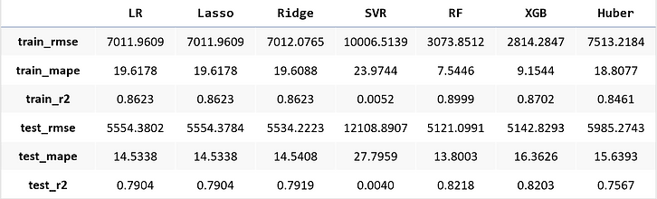
We improved our model in R-Squared significantly:

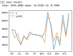
Linear Regression: from R-Squared = 0.6175 -> 0.7904
Lasso: from R-Squared = 0.6175 -> 0.7904
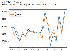
Ridge: from R-Squared = 0.6095 -> 0.7919
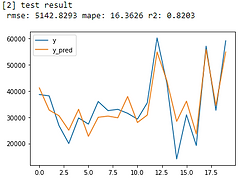
Random Forest: from R-Squared = 0.6898 -> 0.8218
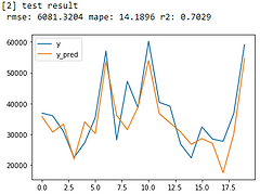
XGBoost: from R-Squared = 0.7029 -> 0.8203
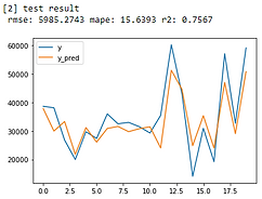
Huber Regression: from R-Squared = 0.2256 -> 0.7567

From error metrics of each model shown below, the result shows that the Random Forest Model has the lowest RMSE and MAPE and the highest R-squared. From the line chart of the random forest, it is also shown that the trend of the predicted value of the orange line is similar to the trend of the present value of the gray line.Therefore, we decided to choose the Random Forest Model to be the predictive model for our COD concentration reduction project.

In [22]:

train_result = pd.DataFrame()

for i,model in enumerate(models):
print('(%d)'%(i+1), model.fit(X_train,y_train))

# train

Linear Regression

Lasso

Ridge

SVR

Random Forest

XGBoost

Huber Regression

Optimization : find a set of parameters for the manufacturing production process to get optimized minimal COD concentration result

After deciding the best predictive model, we need to determine a set of parameters that would be the manufacturing input to get optimized COD concentration. We used PSO Optimization (Particle Swarm Optimization) to get the ideal parameter set in this practice.

The features (input) can be categorized into two types: controllable factors and non-controllable factors. Controllable factors are features which we can adjust the manufacturing set-point value; in contrast, non-controllable are those we cannot. Therefore, we need to confirm the controllable factors and use PSO optimization to get best set-point parameter for the manufacturing process.

According to the site engineers, only 3PIC023.PV and 3FIC014 are controllable factors and the rest are non-controllable ones. Below is the process about how I got the optimized manufacturing set-point values of the two controllable factors.

In [23]:

# Particle Swarm Optimization

from pyswarm import pso

def pso_try(x):
target_num = 30000
# y_target = model.predict(stand_scaler.transform([[0.4,2500,1050,62,280,68,0.85]]))

# x[0] refers to 3PIC023.PV, x[1] refers to 3FIC014,

# the rest of the values are the mean of each features respectively: 3FIC020.PV, 3TI015-1, yield, 3FIC023.PV
y_target = model.predict(stand_scaler.transform([[x[0],x[1],1050,62,280,68,0.85]])) #'model' is Random Forest model
e_target = abs(target_num - y_target)
print(e_target)
return e_target

In [23]:

# Setting upper and lower bound for target controllable factors

x_lb = [0.2,2400]
x_ub = [0.6,2600]

In [23]:

# Start searching for the optimized parameter set and target value

x_opt,y_opt = pso(pso_try,x_lb,x_ub,maxiter = 2,swarmsize=100)

x_opt,y_opt

(array([ 0.6 , 2502]), array([671.98]))

In [23]:

# print optimized target COD value

model.predict(stand_scaler.transform([[x_opt[0],x_opt[1],1050,62,280,68,0.85]]))

array([30671.98])

From the result, we got 0.6 and 2502 as manufacturing set-point value for controllable factors, 3PIC023.PV and 3FIC014, respectively, and expected to reach optimal minimal (30671) of COD concentration.

I discussed this result with the site engineers and after they adjust those two controllable factors to the set-point value as suggestion, the COD concentration successfully dropped from 45000 ppm to approximately 30000 ppm. This practice helped save a large amount on wastewater treatment costs and benefits both the company and the environment.

This successful experience had deepened my enthusiasm for data science; meanwhile, it also reminded me that there are still lots of knowledge, theories and algorithms that I need to learn.

Acerca de

COD Reduction

In Wastewater

AI Project

Motivation

Problems

How to measure the pollutants

# Ｗhat is COD?

Take Actions

Manufacturing Process Introduction

Modeling process

Data Cleaning

Exploratory Data Analysis

Data Transformation

Feature Engineering

Predictive Modeling

Import packages

In [1]:

In [2]:

Input Data

In [3]:

In [4]:

In [5]:

In [6]:

Define Evaluation Metrics

In [7]:

◼ Build a base model

In [8]:

In [9]:

In [10]:

Data Exploration

In [11]:

In [12]:

In [13]:

In [14]:

In [15]:

In [16]:

Data transformation & feature engineering

In [17]:

In [18]:

In [19]:

In [20]:

In [21]:

Results: Modeling & optimization

In [22]:

In [23]:

In [23]:

In [23]:

In [23]:

Data
Cleaning

Exploratory
Data Analysis

Data
Transformation

Feature
Engineering

Predictive
Modeling

Data transformation
& feature engineering